Semi-Supervised Anomaly Detection
I used to think anomaly detection was just an unsupervised learning technique, unsuitable when labeled datasets were available. However, that was a misconception. Some recent readings on anomaly detection have changed my perspective. It turns out anomaly detection can be a good, and sometimes the best, solution in practice—even when labeled data is available.
According to the availability of the data, we divide the anomaly detection (AD) into three parts.
- Unsupervised AD trains a model on a dataset without any annotations (labels), which outputs an anomaly score for each sample.
- Supervised AD trains a model on a fully annotated dataset. We can regard it as a classification model.
- Semi-supervised AD trains a model on a partially annotated dataset to identify anomaly samples.
In practice, it’s common to have a large amount of unlabeled data and only a small set of labeled data. This happens for several reasons. For instance, labeled data is often much more expensive and harder to access than unlabeled data. Additionally, datasets can be imbalanced, with only a limited number of anomaly samples. In such cases, semi-supervised AD becomes an invaluable tool.
It’s also worth noting that AD methods are not restricted to anomaly detection problems. They can be effectively applied to imbalanced classification tasks as well, where minorities are the anomalies.
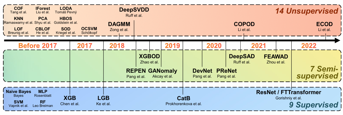
[1] provided 30 benchmark datasets and evaluated 30 anomaly detection (AD) algorithms. The most interesting aspect, in my view, is their experiments on various percentages of labeled anomalies, which reflect different levels of data availability in practice. The figure below illustrates the performance of each algorithm under different data availability scenarios.
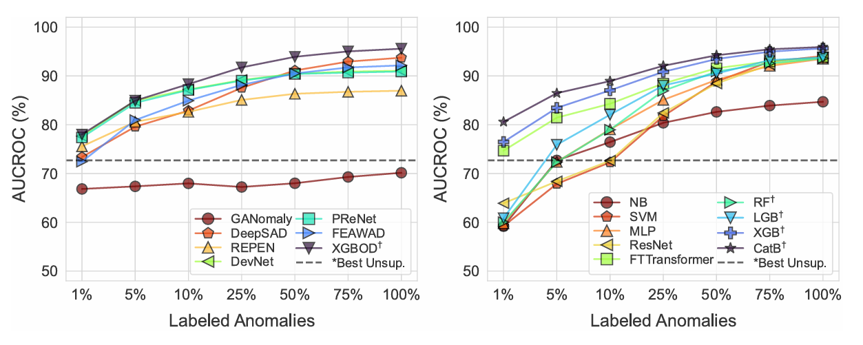
In the figure, the left side shows semi-supervised algorithms, while the right side shows fully supervised algorithms. Here are some noteworthy observations—not necessarily the same as those discussed in the paper [1].
- CatBoost, a supervised method, outperforms all semi-supervised AD methods even when only 1% of labels are available. This suggests that, despite limited annotations, some supervised methods are still worth considering.
- Unsupervised methods struggle to outperform semi-supervised or fully supervised methods when only 1% of labels are available. Labels are the most valuable resource for the model. Instead of focusing solely on model selection, consider strategies to incorporate more labeled data.
- PReNet and XGBOD demonstrate superior performance among semi-supervised AD algorithms, particularly when labeled anomalies are below 10%.
XGBOD
The XGBOD (Extreme Gradient Boosting Outlier Detection) framework combines unsupervised outlier detection and supervised learning in a semi-supervised ensemble approach. The main idea is to enhance the feature space by including outlier scores generated by unsupervised detectors. These enriched features are then used in a supervised learning model, specifically XGBoost, to improve prediction performance.
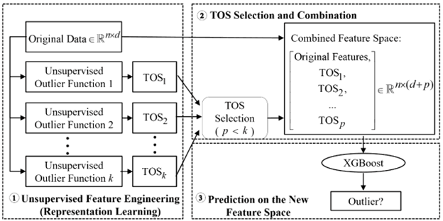
The algorithm operates in three main phases:
Unsupervised Representation Learning. Given a dataset X of n points with d features, apply k unsupervised outlier detection methods to produce transformed outlier scores (TOS).
Transformed Outlier Scores (TOS) Selection. Prune the TOS to retain only the most useful representations. We want to balance diversity and accuracy by using a discounted accuracy function:
\[\Psi(\Phi_i) = \text{Accuracy}(\Phi_i) \big/ \sum_{j \in S} \rho(\Phi_i, \Phi_j)\]where \(S\) is the selected set of TOS, \(\rho(\Phi_i, \Phi_j)\) measures correlation between TOS \(\Phi_i\) and \(\Phi_j.\) The diversity is encouraged by forcing the selected TOS to be less correlated with each other.
Supervised Learning with XGBoost. Train an XGBoost classifier on the refined feature space that includes both the selected TOS and the original feature set X. Do further feature selection using the feature importance mechanism if needed.
PReNet
PReNet (Pairwise Relation prediction Network) is another anomaly detection algorithm that uses a small labeled anomaly set and a large unlabeled dataset. It differs from other algorithms that it takes two samples as inputs, instead of one, and then outputs their relationships.
The samples can be normal or anomaly samples, and thus we have three pairwise relations: 1) anomaly-anomaly (AA), 2) anomaly-unlabeled (AU), and 3) unlabeled-unlabeled (UU). We regard all unlabeled samples as normal samples. Then the relation prediction is formulated as a three-way ordinal regression task. The biggest advantage of such a setting is the data augmentation. Although there are only a few anomaly samples, we can have tons of sample pairs.
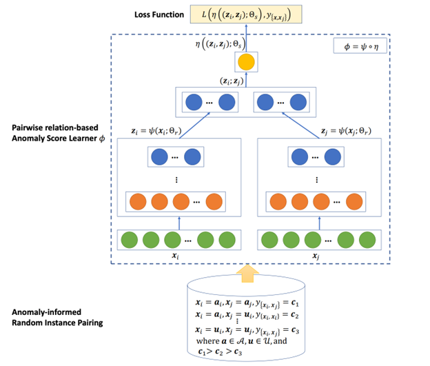
Model architecture. Since PReNet is a pair-wised model, its architecture inherently includes a siamese network to extract features from both samples, and a scoring network that concatenates extracted features of the paired samples and computes anomaly scores for the sample pair.
Model training. After generating sample pairs, its training is like a regular supervised regression training using gradient descent.
Inference. Since it’s a pairwise model, when we want to do inference on a new sample, we need to use the samples in the training data to make it a pair. To make the prediction more robust, we take E normal samples and E anomaly samples, instead of 1 sample from the training data to do an ensemble. Specifically, \(\text{anomalyScore}(x)=\frac{1}{E}(\sum_{i=1}^{E}\phi(a_i, x)+\sum_{j=1}^{E}\phi(u_j, x))\) where \(a_i\) and \(u_j\) are the known anomalies and normal samples.
DeepSAD
DeepSAD (Deep Semi-Supervised Anomaly Detection) does not perform best in the experiments of [1], but its main idea is pretty interesting and convincing.
As a semi-supervised anomaly detection model, DeepSAD also leverages both labeled and unlabeled data. Unlike end-to-end models, DeepSAD maps the features of a sample to a latent space, and then we use the latent features to compute an anomaly score.
DeepSAD does not rely on a specific architecture, as long as the network can map inputs to a latent space. Instead, its uniqueness lies in its objective function and training process.
Objective function. The objective function includes three terms.

-
In the first term, we pull all unlabeled samples to the center c in the latent space. This is because we assume most unlabeled data are normal and the normal data share a similar pattern. Therefore most unlabeled data should stay close in the latent space.
-
In the second term, we pull all known normal samples (y=+1) to the center c as well. Additionally, we push the known anomalies (y=-1) away from the center c.
-
The third term is for regularization.
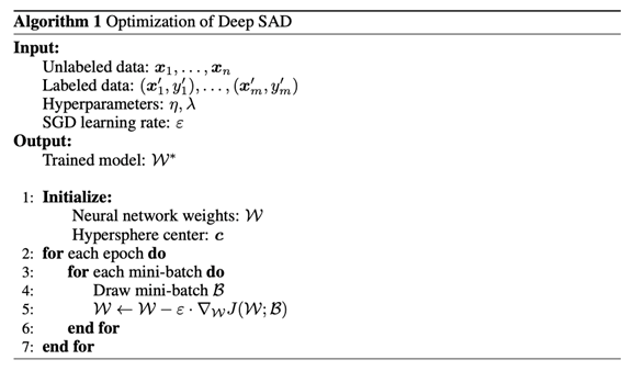
Training Process. We can train DeepSAD in three phases.
- Pretrain the network as an autoencoder using reconstruction loss to learn robust initial features. The autoencoder pre-training is not necessary but it ensures stable initialization.
- Initialize the hypersphere center c as the mean of the latent representations of normal data, by feeding the known normal data into the pre-trained autoencoder.
- Use stochastic gradient descent to optimize the objective
References
[1] Han, S., Hu, X., Huang, H., Jiang, M., & Zhao, Y. (2022). Adbench: Anomaly detection benchmark. Advances in Neural Information Processing Systems, 35, 32142-32159. https://arxiv.org/abs/2206.09426
[2] Zhao, Y., & Hryniewicki, M. K. (2018, July). Xgbod: improving supervised outlier detection with unsupervised representation learning. In 2018 International Joint Conference on Neural Networks (IJCNN) (pp. 1-8). IEEE. https://arxiv.org/abs/1912.00290
[3] Pang, G., Shen, C., Jin, H., & van den Hengel, A. (2023, August). Deep weakly-supervised anomaly detection. In Proceedings of the 29th ACM SIGKDD Conference on Knowledge Discovery and Data Mining (pp. 1795-1807). https://arxiv.org/abs/1910.13601
[4] Ruff, L., Vandermeulen, R. A., Görnitz, N., Binder, A., Müller, E., Müller, K. R., & Kloft, M. (2019). Deep semi-supervised anomaly detection. arXiv preprint arXiv:1906.02694. https://arxiv.org/abs/1906.02694