Double Machine Learning for Pricing Elasticity Estimation
What is pricing elasticity
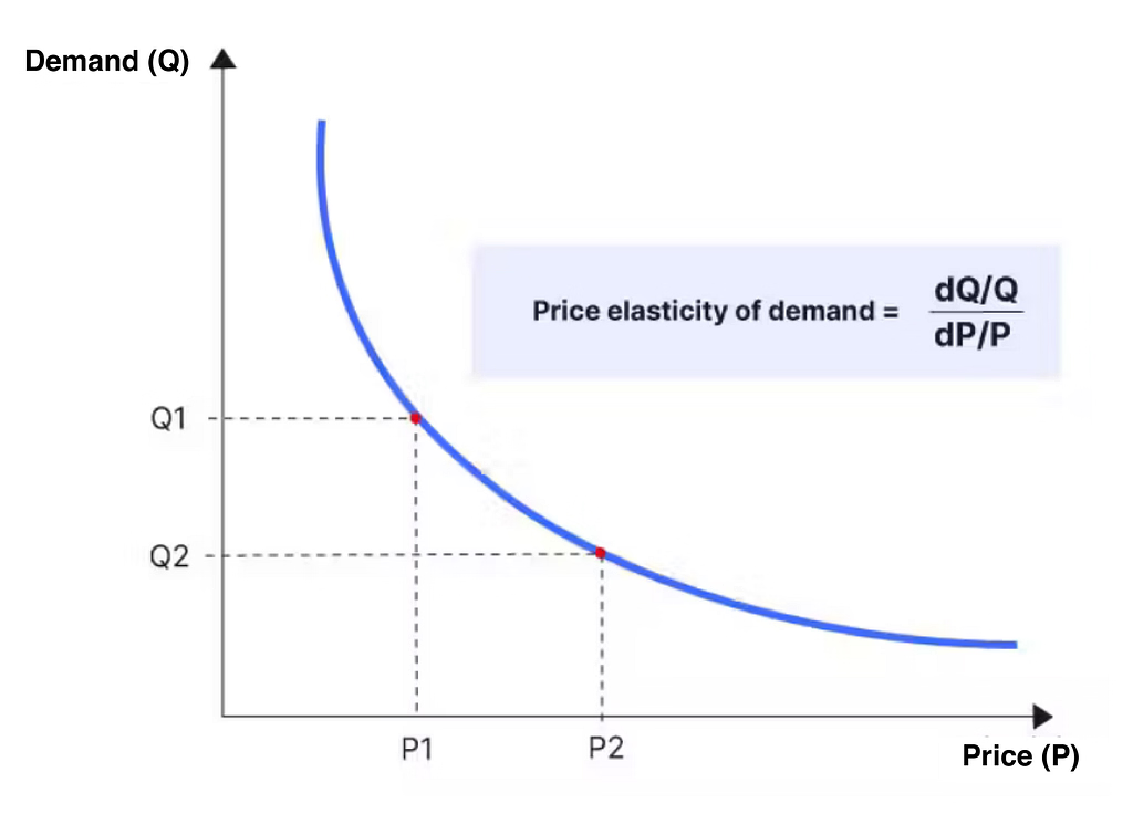
Pricing elasticity describes the sensitivity of demand to changes in price for a particular product. When demand is more elastic, an increase in price will result in a greater reduction in demand. This concept allows businesses to estimate how many more units of a product they could sell if they were to lower the price by a certain percentage.
In short, economists summarized the elasticity to be a simple equation:
\[\theta = \frac{\partial Q / Q}{\partial P / P}\]or equivalently,
\[log Q \sim \theta log P\]where \(P\) is price, \(Q\) is demand, and \(\theta\) is the elasticity. This equation tells us that given a percent change of price (\(P\)), the percent change of demanded quantity (\(Q\)) is a constant. This constant is the elasticity, \(\theta\).
The basic idea is that a \$1 increase in price will have a larger impact on demand for a product that costs \$5 compared to one that costs \$100. Consumers tend to care about relative changes rather than absolute changes. This definition is convenient because it allows the parameter \(\theta\) to remain constant as the price changes. With a reliable estimate of \(\theta\), a retailer can make counterfactual predictions about their prices, such as “if I were to increase the price of my product by 5%, I could sell 5θ% more units” (usually \(\theta\) is negative).
A good elasticity estimation can be very important to a retailer in many scenarios:
-
Pricing Strategy: A retailer with a good understanding of price elasticity can optimize their pricing strategy to maximize revenue. For example, if a product has low elasticity, the retailer can increase the price without worrying too much about a decrease in demand. On the other hand, for a highly elastic product, lowering the price might lead to a significant increase in demand, leading to higher revenue overall.
-
Promotional Offers: Retailers can use price elasticity to determine the best promotional offers for their products. For instance, if a product has high elasticity, a small discount might result in a big increase in demand. However, for a product with low elasticity, a larger discount might be necessary to encourage consumers to buy.
-
Inventory Management: Retailers can use price elasticity to help manage their inventory. For example, if they know that a product is highly elastic and likely to sell out quickly if the price is lowered, they may decide to keep a smaller inventory and replenish it more frequently.
-
Market Analysis: By examining price elasticity across different products and markets, a retailer can gain insights into consumer behavior and preferences. This information can be used to inform pricing, marketing, and product development decisions.
Why do we need double ML for pricing elasticity estimation
Although a good elasticity estimation can be very important to a retailer, it is challenging to estimate the pricing elasticity coefficient in the real world.
We probably want to estimate elasticity from historical selling data. But historical selling data can lead to a biased elasticity if we do not remove the confounding factors, for example, holidays. In many industries, low prices are associated with low sales. For example, in the hotel industry, prices are low outside the tourist season, and prices are high when demand is highest, and hotels are full. Given that data, a naive estimation might suggest that increasing the price would lead to more sales.

To remove the confounding effects, the most straightforward way is to set up a randomized experiment. For instance, a retailer could randomly adjust product prices up and down or even randomize prices across different customers. Then with the collected price and demand data, we are easily able to estimate the pricing elasticity. However, this type of experimentation is not good or realistic.
- The experiment is expensive as it requires selling products at suboptimal prices and can negatively impact the customer experience.
- Usually, a short experiment might not be generalizable to other seasons or holidays.
Given the non-randomized observations, how do we remove the confounding effects and estimate the true effect of price on sales? The answer is Double Machine Learning (DML).
How does double ML work
Pricing elasticity estimation is not just fitting a machine learning model using the available data. As we said in the last section, a naive estimation may give ridiculous suggestions due to biased data.
Double machine learning is a method that combines machine learning algorithms to estimate treatment effects in causal inference. It aims to answer the questions of ‘what if’. For example, what sales would be if I set the discount to 30%?
Generally, DML includes two phases. 1) In the first phase, we train two separate models to predict the treatment (price) and outcome (sales) using confounding variables, respectively. 2) In the second phase, we estimate the pricing elasticity on the residuals of price and sales from the trained models.
Specifically, we want to estimate the causal effect, \(\theta\), using the following equations:
\[Y = \theta T + G(W) + \epsilon\]where \(W\) is the confounding variables that can impact both \(Y\) and \(T\).
This equation holds after transformation:
\[Y-E[Y\vert W] = \theta (T - E[T\vert W]) + \epsilon\]It tells us that, if we can build two models to estimate \(E[Y\vert W]\) and \(E[T\vert W]\), then we are able to derive the treatment effect from the regression on residuals. Actually this is Frisch-Waugh-Lovell (FWL) theorem!
Based on FWL theorem, DML estimates treatment effect through the following procedures:
- Estimate the outcome \(Y\) with confounding variables \(W\) using a flexible ML regression model \(M_y\).
- Estimate the treatment \(T\) with features confounding variables \(W\) using a flexible ML regression model \(M_t\).
- Obtain the residuals \(\tilde{Y}=Y-M_y(W)\) and \(\tilde{T}=T-M_t(W)\).
- Regress the residuals of the outcome on the residuals of the treatment \(\tilde{Y}=\theta \tilde{T}+\epsilon\)
In the case of pricing elasticity, we simply replace \(Y\) with \(log Q\) and replace \(T\) with \(log P\). To give some intuition, after we predict Price (\(log P\)) from confounding variables (\(W\), e.g. is_holiday), we will get a residual, \(\tilde{log P}\), which is uncorrelated with all confounding variables.
In this way, we obtain a pricing elasticity \(\theta\) with confounding variables controlled. In the example of hotels, we are able to get the true elasticity with is_tourist_season controlled. The impact of the tourist season has been removed in Step 1 and Step 2.
Elasticity estimation in real world
In the real world, we usually face an even worse situation than the confounding effects, which is insufficient data. Usually, we take common strategies, such as regularization, ensemble learning, and cross-validation. There are more things we can do for elasticity estimation, actually.
Suppose we are going to estimate the elasticity for a new product with only 1-week selling history. It is impossible to obtain a reliable elasticity with such limited data. But we have some similar products with long selling history. Using the data of similar products can partially solve the data insufficiency.
- The first strategy is to estimate the elasticities of those similar products and take the average or weighted average. The weights can be defined as the similarities between the new product and old products.
- If there are some product-level factors that can impact the elasticity of the product, \(X\), such as product color, we can fit all products together in a single model. We just need to induce them into the model by setting \(\theta = \theta(X) = X \dot \beta\), where \(X\) is the factors that impact the elasticity, and \(\beta\) is the corresponding coefficients. See this article [1] for the details.
References
[1] https://matheusfacure.github.io/python-causality-handbook/22-Debiased-Orthogonal-Machine-Learning.html
[2] https://towardsdatascience.com/causal-inference-example-elasticity-de4a3e2e621b
[3] https://doi.org/10.1016/j.eswa.2013.07.059
[4] https://arxiv.org/pdf/2205.01875.pdf
[5] https://www.actable.ai/use-cases/optimizing-sales-causal-inference-could-be-your-secret-sauce
[6] https://github.com/larsroemheld/causalinf_ex_elasticity/blob/main/elasticity_dml.ipynb